3  优雅的处理数据

对于工程实践而言，我们需要一套既具备高可读性，又能应对大规模计算的数据处理流。本节我们将从数据处理的“语法”出发，探讨如何通过分箱技术让线性模型具备非线性表达能力，并最终使用 data.table 突破性能瓶颈。

3.1 数据处理的语法

传统的数据清洗往往伴随着大量嵌套的函数和临时变量，代码逻辑很难梳理清楚。Hadley Wickham 提出的 tidyverse 体系，其核心贡献在于确立了一套数据处理的语法（A Grammar for Data Wrangling）。它将数据操作抽象为一系列直观的动词组合：

• 选择（select）：选取变量列
• 筛选（filter）：筛选行，样本
• 变形（mutate）：增加或者修改变量
• 汇总（summarize）：一般和 group_by() 连用，表示根据某一列做汇总。如果单独使用则是全局汇总。
• 排序（arrange）：按照规则排序

通过引入原生管道符号 |>（或 magrittr 的 %>%），复杂的逻辑被顺畅地拆解为人类可读的数据流。构建统计分析/机器学习/深度学习前置的预处理流水线（Preprocessing Pipeline）。

library(tidyverse)
library(knitr)

# 模拟一张用户属性表
set.seed(123)
raw_users <- tibble(
  user_id = 1:100,
  region = sample(c("华东", "华北", "华南", "西南"), 100, replace = TRUE),
  age = sample(c(18:70, NA), 100, replace = TRUE)
)

tibble 是 tidyverse 对传统 data.frame 的现代化改进版本。它遵循 tidy data 理念，提供更一致、更可预测的行为：不会自动转换字符串为因子，不会在子集操作时自动降维，也不会因为列名冲突而悄悄修改变量类型。这种“类型稳定性”让数据处理过程更安全、更透明。

与 data.frame 相比，tibble 的打印方式更友好：默认只显示前几行，并对宽列进行截断，便于快速浏览数据结构而不刷屏。它还与 tidyverse 的 dplyr、tidyr、ggplot2 等包深度整合，成为整个 tidyverse 数据分析流程的基础数据结构。总体来说，tibble 强调可读性、稳定性和管道友好性，使数据处理代码更清晰、更易维护，是现代 R 数据分析的推荐默认格式。

我们将 raw_users 做一个简单的示例统计分析：

raw_users |>
  group_by(region) |>
  summarise(
    mean_age = mean(age, na.rm = TRUE),
    cnt = n()
  )

# A tibble: 4 × 3
  region mean_age   cnt
  <chr>     <dbl> <int>
1 华东       46.6    28
2 华北       46.5    26
3 华南       45.9    29
4 西南       39.7    17

或者我们做一个交叉列联表：

result <- raw_users |>
  drop_na(age) |> 
  filter(age >= 18) |> 
  mutate(age_group = case_when(
    age < 30 ~ "年轻 (18-29)",
    age < 50 ~ "中年 (30-49)",
    TRUE ~ "资深 (50+)"
  )) |>
  group_by(region, age_group) |>
  summarise(
    cnt = n(),
    .groups = "drop"
  )
result

# A tibble: 12 × 3
   region age_group      cnt
   <chr>  <chr>        <int>
 1 华东   中年 (30-49)    12
 2 华东   年轻 (18-29)     4
 3 华东   资深 (50+)      10
 4 华北   中年 (30-49)    10
 5 华北   年轻 (18-29)     5
 6 华北   资深 (50+)      11
 7 华南   中年 (30-49)    15
 8 华南   年轻 (18-29)     4
 9 华南   资深 (50+)      10
10 西南   中年 (30-49)     6
11 西南   年轻 (18-29)     4
12 西南   资深 (50+)       5

把长表（long）变为宽表（wide）：

result |>
  pivot_wider(
    names_from = age_group,
    values_from = cnt,
    values_fill = 0   # 缺失填 0（可选）
  )

# A tibble: 4 × 4
  region `中年 (30-49)` `年轻 (18-29)` `资深 (50+)`
  <chr>           <int>          <int>        <int>
1 华东               12              4           10
2 华北               10              5           11
3 华南               15              4           10
4 西南                6              4            5

3.2 连表操作

真实业务场景的数据通常散落在不同的数据库表中。tidyverse 提供了类似 SQL（Structured Query Language，结构化查询语言，用于管理关系型数据库的查询语言）的 Join 动词（如 left_join(), inner_join()），使得多表关联也能完美融入管道操作中，保持代码的连贯性。

# 模拟一张订单表
raw_orders <- tibble(
  user_id = sample(1:100, 150, replace = TRUE),
  amount = runif(150, 50, 2000)
)

模拟一个场景：用户信息同订单信息联合起来，汇总统计用户相关的信息：

result <- raw_users |>
  drop_na(age) |> 
  filter(age >= 18) |> 
  mutate(age_group = case_when(
    age < 30 ~ "年轻 (18-29)",
    age < 50 ~ "中年 (30-49)",
    TRUE ~ "资深 (50+)"
  )) |>
  left_join(raw_orders, by = "user_id") |> 
  replace_na(list(amount = 0)) |> 
  group_by(region, age_group) |> 
  summarize(
    total_amount = sum(amount),
    avg_amount = mean(amount),
    n_users = n(),
    .groups = "drop"
  ) |> 
  arrange(region, age_group) |>
  mutate(
    status = case_when(
      n_users > 20 ~ "Completed",
      n_users < 7 ~ "Delayed",
      TRUE ~ "In Progress"
    )
  )

library(gt)
library(gtExtras)
result |>
  gt() |>
  tab_options(
    table.font.size = gt::px(14)
  )

region	age_group	total_amount	avg_amount	n_users	status
华东	中年 (30-49)	16674.330	757.9241	22	Completed
华东	年轻 (18-29)	4412.615	630.3735	7	In Progress
华东	资深 (50+)	18954.548	997.6078	19	In Progress
华北	中年 (30-49)	17855.603	939.7686	19	In Progress
华北	年轻 (18-29)	5594.903	799.2719	7	In Progress
华北	资深 (50+)	15444.079	812.8463	19	In Progress
华南	中年 (30-49)	11196.559	533.1695	21	Completed
华南	年轻 (18-29)	10215.918	1276.9898	8	In Progress
华南	资深 (50+)	19029.024	1001.5276	19	In Progress
西南	中年 (30-49)	6481.338	648.1338	10	In Progress
西南	年轻 (18-29)	3984.428	664.0713	6	Delayed
西南	资深 (50+)	12097.703	1099.7912	11	In Progress

使用 gt 包将该表格重构为符合大众阅读习惯的样式（如 ESPN 表格样式）：

result_table <- result |>
  gt(groupname_col = "region", id = "sales_report") |>
  gt_theme_espn() |>
  
  tab_header(
    title = md("**区域用户消费行为深度透视**"),
    subtitle = md("*基于年龄分层的订单贡献度及进度追踪*")
  ) |>
  
  cols_label(
    age_group = "年龄画像",
    total_amount = "消费总额 (趋势图)",
    avg_amount = "人均消费",
    n_users = "覆盖人数",
    status = "当前状态" # 【新增】标签映射
  ) |>
  
  fmt_currency(
    columns = avg_amount,
    currency = "CNY",
    decimals = 1
  ) |>
  
  gt_plt_bar_pct(
    column = total_amount, 
    fill = "#1498db",        
    background = "#e5e5e5",  
    scaled = FALSE,          
    labels = TRUE,           
    decimals = 1,            
    label_cutoff = 0
  ) |>
  # 1. Completed 状态：浅绿背景 + 深绿加粗字体
  tab_style(
    style = cell_fill(color = "#e6fffa"),
    locations = cells_body(columns = status, rows = status == "Completed")
  ) |>
  tab_style(
    style = cell_text(color = "#38a169", weight = "bold"),
    locations = cells_body(columns = status, rows = status == "Completed")
  ) |>
  # 2. Delayed 状态：红色加粗字体
  tab_style(
    style = cell_text(color = "#e53e3e", weight = "bold"),
    locations = cells_body(columns = status, rows = status == "Delayed")
  ) |>
  # 3. In Progress 状态：橙黄色加粗字体 (补充设计，保持视觉平衡)
  tab_style(
    style = cell_text(color = "#d69e2e", weight = "bold"),
    locations = cells_body(columns = status, rows = status == "In Progress")
  ) |>

  tab_style(
    style = cell_text(weight = "bold", color = "#2c3e50", size = px(14)),
    locations = cells_row_groups()
  ) |>
  
  tab_style(
    style = gt::cell_text(size = gt::px(14)),
    locations = gt::cells_body()
  ) |>
  
  gt_color_rows(
    columns = avg_amount, 
    palette = "Greens", 
    alpha = 0.5,
    domain = range(result$avg_amount)
  ) |>
  
  # 将 n_users 和 status 列都居中对齐，排版更整洁
  cols_align(align = "center", columns = c(n_users, status)) |>
  
  tab_options(
    table.width = px(550), # 稍微加宽表格以容纳新列
    data_row.padding = px(3),
    heading.align = "left",
    table.border.top.style = "none"
  ) |>
  
  tab_source_note(
    source_note = md("*注：消费总额趋势条根据各区域最大值自动缩放*")
  )

result_table

区域用户消费行为深度透视
基于年龄分层的订单贡献度及进度追踪
年龄画像	消费总额 (趋势图)	人均消费	覆盖人数	当前状态
华东
中年 (30-49)	87.6%	¥757.9	22	Completed
年轻 (18-29)	23.2%	¥630.4	7	In Progress
资深 (50+)	99.6%	¥997.6	19	In Progress
华北
中年 (30-49)	93.8%	¥939.8	19	In Progress
年轻 (18-29)	29.4%	¥799.3	7	In Progress
资深 (50+)	81.2%	¥812.8	19	In Progress
华南
中年 (30-49)	58.8%	¥533.2	21	Completed
年轻 (18-29)	53.7%	¥1,277.0	8	In Progress
资深 (50+)	100%	¥1,001.5	19	In Progress
西南
中年 (30-49)	34.1%	¥648.1	10	In Progress
年轻 (18-29)	20.9%	¥664.1	6	Delayed
资深 (50+)	63.6%	¥1,099.8	11	In Progress
注：消费总额趋势条根据各区域最大值自动缩放

3.3 快速数据分析

skimr 是一个非常强大且受欢迎的 R 包，主要用于探索性数据分析 (EDA)。它的核心功能是快速生成数据框 (Data Frame) 的摘要统计信息，通常被 R 语言使用者视为基础包中 summary() 函数的“超级升级版”。

• 它能在 R 控制台 (Console) 中直接打印出微型直方图（针对数值型变量）和微型条形图。可以直接观察数据的分布偏态。
• 自动将变量按类型（如：数值型 numeric、字符型 character、因子 factor、逻辑型 logical、日期型 Date 等）分类显示。
• 清晰地列出每个变量的缺失值数量 (n_missing) 以及数据的完整率 (complete_rate)，方便在建模前处理空值。
• 可以无缝使用 dplyr 的管道符 (%>% 或 |>)、group_by() 和 filter() 等函数对统计结果进行二次操作。

# 加载所需的 EDA 包 (如果没有请先 install.packages)
library(tidymodels)
library(tidyverse)
library(torch)
library(skimr)
data(ames)
# 所有的 EDA 都应该只在训练集上做，防止数据泄露（Data Leakage）！
set.seed(123)
torch_manual_seed(123)
ames_split <- initial_split(ames, prop = 0.80)
ames_train <- training(ames_split)

# 1. 极速扫描全表 (看一眼控制台输出，极其惊艳)
ames_train %>%
  skim_without_charts() %>%
  # 直接剔除指定的列
  select(-n_missing, -complete_rate)

Data summary

Name	Piped data
Number of rows	2344
Number of columns	74
_______________________
Column type frequency:
factor	40
numeric	34
________________________
Group variables	None

Variable type: factor

skim_variable	ordered	n_unique	top_counts
MS_SubClass	FALSE	16	One: 851, Two: 455, One: 226, One: 158
MS_Zoning	FALSE	7	Res: 1813, Res: 376, Flo: 109, Res: 22
Street	FALSE	2	Pav: 2334, Grv: 10
Alley	FALSE	3	No_: 2188, Gra: 92, Pav: 64
Lot_Shape	FALSE	4	Reg: 1479, Sli: 789, Mod: 63, Irr: 13
Land_Contour	FALSE	4	Lvl: 2112, HLS: 98, Bnk: 87, Low: 47
Utilities	FALSE	3	All: 2341, NoS: 2, NoS: 1
Lot_Config	FALSE	5	Ins: 1706, Cor: 426, Cul: 140, FR2: 61
Land_Slope	FALSE	3	Gtl: 2227, Mod: 104, Sev: 13
Neighborhood	FALSE	28	Nor: 362, Col: 224, Old: 196, Edw: 160
Condition_1	FALSE	9	Nor: 2012, Fee: 125, Art: 76, RRA: 44
Condition_2	FALSE	8	Nor: 2319, Fee: 11, Art: 4, Pos: 3
Bldg_Type	FALSE	5	One: 1924, Twn: 190, Dup: 95, Twn: 82
House_Style	FALSE	8	One: 1193, Two: 687, One: 250, SLv: 106
Overall_Cond	FALSE	9	Ave: 1339, Abo: 427, Goo: 298, Ver: 107
Roof_Style	FALSE	6	Gab: 1853, Hip: 443, Gam: 19, Fla: 16
Roof_Matl	FALSE	7	Com: 2310, Tar: 19, WdS: 7, WdS: 5
Exterior_1st	FALSE	16	Vin: 805, Met: 365, HdB: 362, Wd : 329
Exterior_2nd	FALSE	17	Vin: 793, Met: 363, HdB: 336, Wd : 316
Mas_Vnr_Type	FALSE	5	Non: 1420, Brk: 701, Sto: 199, Brk: 23
Exter_Cond	FALSE	5	Typ: 2043, Goo: 232, Fai: 59, Exc: 7
Foundation	FALSE	6	PCo: 1027, CBl: 1012, Brk: 252, Sla: 41
Bsmt_Cond	FALSE	6	Typ: 2090, Goo: 99, Fai: 81, No_: 69
Bsmt_Exposure	FALSE	5	No: 1531, Av: 331, Gd: 226, Mn: 184
BsmtFin_Type_1	FALSE	7	Unf: 684, GLQ: 683, ALQ: 341, Rec: 218
BsmtFin_Type_2	FALSE	7	Unf: 1993, Rec: 83, LwQ: 74, No_: 70
Heating	FALSE	6	Gas: 2306, Gas: 22, Gra: 8, Wal: 5
Heating_QC	FALSE	5	Exc: 1175, Typ: 707, Goo: 383, Fai: 76
Central_Air	FALSE	2	Y: 2176, N: 168
Electrical	FALSE	6	SBr: 2146, Fus: 147, Fus: 41, Fus: 8
Functional	FALSE	8	Typ: 2181, Min: 54, Min: 52, Mod: 30
Garage_Type	FALSE	7	Att: 1380, Det: 635, Bui: 135, No_: 130
Garage_Finish	FALSE	4	Unf: 987, RFn: 639, Fin: 586, No_: 132
Garage_Cond	FALSE	6	Typ: 2121, No_: 132, Fai: 64, Poo: 13
Paved_Drive	FALSE	3	Pav: 2116, Dir: 176, Par: 52
Pool_QC	FALSE	5	No_: 2335, Exc: 3, Goo: 3, Typ: 2
Fence	FALSE	5	No_: 1880, Min: 275, Goo: 91, Goo: 88
Misc_Feature	FALSE	6	Non: 2254, She: 81, Gar: 4, Oth: 3
Sale_Type	FALSE	10	WD : 2032, New: 185, COD: 74, Con: 20
Sale_Condition	FALSE	6	Nor: 1937, Par: 188, Abn: 158, Fam: 34

Variable type: numeric

skim_variable	mean	sd	p0	p25	p50	p75	p100
Lot_Frontage	57.58	33.17	0.00	43.00	63.00	78.00	313.00
Lot_Area	10124.68	8302.84	1300.00	7347.50	9350.00	11553.75	215245.00
Year_Built	1971.25	30.09	1872.00	1954.00	1973.00	2000.00	2010.00
Year_Remod_Add	1983.91	20.91	1950.00	1965.00	1992.00	2004.00	2010.00
Mas_Vnr_Area	100.78	179.29	0.00	0.00	0.00	162.00	1600.00
BsmtFin_SF_1	4.18	2.23	0.00	3.00	3.00	7.00	7.00
BsmtFin_SF_2	49.88	169.34	0.00	0.00	0.00	0.00	1474.00
Bsmt_Unf_SF	553.34	438.68	0.00	216.00	460.50	789.00	2336.00
Total_Bsmt_SF	1045.02	445.63	0.00	784.00	988.00	1286.50	6110.00
First_Flr_SF	1153.53	393.78	334.00	872.75	1078.50	1373.25	5095.00
Second_Flr_SF	330.15	427.04	0.00	0.00	0.00	700.25	2065.00
Gr_Liv_Area	1488.75	508.52	334.00	1109.75	1432.00	1734.50	5642.00
Bsmt_Full_Bath	0.43	0.53	0.00	0.00	0.00	1.00	3.00
Bsmt_Half_Bath	0.06	0.25	0.00	0.00	0.00	0.00	2.00
Full_Bath	1.56	0.55	0.00	1.00	2.00	2.00	4.00
Half_Bath	0.37	0.50	0.00	0.00	0.00	1.00	2.00
Bedroom_AbvGr	2.84	0.82	0.00	2.00	3.00	3.00	6.00
Kitchen_AbvGr	1.05	0.22	0.00	1.00	1.00	1.00	3.00
TotRms_AbvGrd	6.41	1.57	2.00	5.00	6.00	7.00	15.00
Fireplaces	0.58	0.65	0.00	0.00	1.00	1.00	4.00
Garage_Cars	1.76	0.76	0.00	1.00	2.00	2.00	5.00
Garage_Area	471.85	216.38	0.00	315.75	480.00	576.00	1418.00
Wood_Deck_SF	93.07	128.63	0.00	0.00	0.00	168.00	1424.00
Open_Porch_SF	46.34	65.48	0.00	0.00	25.00	70.00	547.00
Enclosed_Porch	21.98	60.06	0.00	0.00	0.00	0.00	584.00
Three_season_porch	2.50	24.17	0.00	0.00	0.00	0.00	508.00
Screen_Porch	16.26	55.81	0.00	0.00	0.00	0.00	480.00
Pool_Area	2.00	34.05	0.00	0.00	0.00	0.00	800.00
Misc_Val	52.36	571.44	0.00	0.00	0.00	0.00	17000.00
Mo_Sold	6.23	2.71	1.00	4.00	6.00	8.00	12.00
Year_Sold	2007.79	1.32	2006.00	2007.00	2008.00	2009.00	2010.00
Sale_Price	178985.66	80509.79	12789.00	128000.00	159000.00	211000.00	755000.00
Longitude	-93.64	0.03	-93.69	-93.66	-93.64	-93.62	-93.59
Latitude	42.03	0.02	41.99	42.02	42.03	42.05	42.06

还有一个可以快速做自动化探索性数据分析的的包叫做DataExplorer。

在面对一个完全陌生的新数据集时，写代码逐个变量画图会耗费大量时间。这个包旨在通过极简的代码（通常只有一行），瞬间为你生成海量高质量的统计图表，甚至是一份完整的 HTML 数据诊断报告。

• 它能自动扫描数据集的结构、缺失值、分布和相关性，并打包输出为一个交互式的 HTML 报告。
• 提供了一系列以 plot_ 开头的函数，涵盖了数据科学中 80% 以上的常规可视化需求。
• 在进行机器学习建模前，你可以指定一个“目标变量”（Y值），DataExplorer 会自动分析其他所有特征（X值）与这个目标变量的关系。
• 它的底层绘图逻辑基于 ggplot2，且处理速度优化得很好，同时支持离散型和连续型数据的自动化分类处理。

# 图形未绘制，请同学们自行运行代码
library(DataExplorer) # 批量绘图神器
plot_intro(ames_train)     # 整体结构图：多少连续变量、多少离散变量、多少缺失行
# plot_missing(ames_train)   # 缺失值排行榜（决定哪些列该丢弃，哪些该插补）
# Feature Distributions
# 1. 批量查看所有【连续变量】的分布
plot_histogram(ames_train, nrow = 3L, ncol = 3L)

# 2. 批量查看所有【分类变量】的频数
# 哪些类别的长条极短？需要 step_other(threshold = 0.01) 把它们合并为 "other"
plot_bar(
  ames_train, 
  nrow = 3L, 
  ncol = 3L,
  theme_config = list(
    axis.text.y = element_blank(),  # 隐藏 Y 轴文字
    axis.ticks.y = element_blank()  # 顺便隐藏 Y 轴的刻度线，更干净
  )
)

3.4 连续型数据离散化

观察数据情况，会发现一个问题。像全卫数量 (Full_Bath)、半卫数量 (Half_Bath)、车库可停车辆数 (Garage_Cars) 甚至整体质量评分 (Overall_Qual)，它们在数据字典中确实用数字记录，但它们本质上是离散的分类变量（或有序因子），而不是连续的数值。如果直接放进回归模型里，模型会误以为 2 个浴室是 1 个浴室的绝对两倍，这可能会扭曲业务逻辑。

将这些变量转化为因子类型，并切分数据为 train 和 test：

ames_clean <- ames %>%
  mutate(
    across(
      # 条件：是数值型，且唯一值的数量 <= 10（可以根据需要调整这个阈值）
      where(~ is.numeric(.x) && n_distinct(.x) <= 10), 
      as.factor
    )
  )
ames_split <- initial_split(ames_clean, prop = 0.80)
ames_train <- training(ames_split)
ames_test <- testing(ames_split)

再考虑一种情况：

library(partykit)
ct_demo <- ctree(
  log(Sale_Price) ~ Lot_Frontage,
  data = ames_clean,
  control = ctree_control(
    maxdepth = 3,        # 限制树深度
    minbucket = 20       # 每个叶节点最少样本数
  )
)
plot(ct_demo,
    tp_args = list(      # 截断箱线图的上下 1%，专注显示核心分布区间
    yscale = quantile(log(ames_clean$Sale_Price), c(0.01, 0.99)), 
    cex = 0
  ))

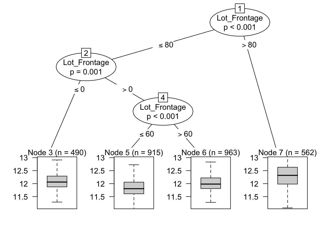
针对于 Lot_Frontage 这个变量，我们将其按照上图分段，对于 outcomes 的预测会更好。

基于此想法，我们引入连续型变量离散化的做法（注意不是均匀分段，而是基于树模型）：

library(tidymodels)
library(embed)
rec <- recipe(Sale_Price ~ ., data = ames_train) %>%
  step_rm(matches("Id|Longitude|Latitude")) %>%
  step_other(all_nominal_predictors(), threshold = 0.01) %>%
  step_nzv(all_predictors()) %>%
#  step_log(Gr_Liv_Area, Lot_Area, base = 10) %>%
  # bins 处理
  step_mutate(
    across(c(where(is.numeric), -Sale_Price), ~ ., .names = "{.col}_bin")) %>%
  step_discretize_cart(
      ends_with("_bin"), 
      outcome = "Sale_Price", 
      tree_depth = 3,             
      cost_complexity = 0.001      
  ) %>%
  # step_rm(where(is.numeric)) %>%   # 本条为错误表达，正确的是下一条。
  step_rm(all_numeric_predictors()) %>%
  # 此时 ends_with("_bin") 里面全都是成功分段的 factor 了
  step_dummy(all_nominal_predictors(), one_hot = TRUE) %>%
  # 接着常规操作
  step_nzv(all_predictors()) %>%
  step_normalize(all_outcomes()) %>%
  step_normalize(all_predictors())


# 重新训练并应用
prep_rec <- prep(rec)
train_df <- bake(prep_rec, new_data = NULL)
test_df  <- bake(prep_rec, new_data = ames_test)

ncol(train_df)      # 查看维度，包括 outcomes

[1] 180

names(train_df) |>  # 打印部分变量
  keep(str_detect, "Sale_Condition|Lot_Frontage_bin")

[1] "Sale_Condition_Abnorml"         "Sale_Condition_Normal"         
[3] "Sale_Condition_Partial"         "Lot_Frontage_bin_X..Inf.10.5." 
[5] "Lot_Frontage_bin_X.10.5.71.5."  "Lot_Frontage_bin_X.71.5.81.5." 
[7] "Lot_Frontage_bin_X.81.5.90.5."  "Lot_Frontage_bin_X.90.5.118.5."

最后使用弹性网来预测：

x_train <- torch_tensor(
  as.matrix(train_df %>% select(-Sale_Price)), dtype = torch_float())
y_train <- torch_tensor(
  matrix(train_df$Sale_Price, ncol=1), dtype = torch_float())

x_test <- torch_tensor(
  as.matrix(test_df %>% select(-Sale_Price)), dtype = torch_float())
y_test <- torch_tensor(
  matrix(test_df$Sale_Price, ncol=1), dtype = torch_float())

model <- nn_sequential(
  nn_linear(ncol(x_train), 128), # 输入特征 -> 128个神经元
  nn_relu(),                     # 激活函数
  nn_linear(128, 64),            # 128 -> 64
  nn_relu(),                     # 激活函数
  nn_linear(64, 1)               # 64 -> 输出1个预测值
)
learning_rate <- 0.0025
optimizer <- optim_adam(model$parameters, lr = learning_rate)
loss_fn <- nn_mse_loss()   # 初始化后使用

n_in <- ncol(x_train)
feature_names <- colnames(train_df %>% select(-Sale_Price))

w <- (torch_randn(n_in, 1) * 0.1)$requires_grad_(TRUE)
b <- torch_zeros(1, requires_grad = TRUE)

lambda <- 0.5
alpha <- 0.95
learning_rate <- 0.002
optimizer <- optim_adam(list(w, b), lr = learning_rate)

# 5. 带有软阈值的训练循环
epochs <- 1000
train_losses <- numeric(epochs)
w_history <- matrix(NA, nrow = epochs, ncol = n_in)
colnames(w_history) <- feature_names

for (t in 1:epochs) {
  optimizer$zero_grad()
  
  y_pred <- torch_mm(x_train, w) + b # 向前传播
  
  mse_loss <- loss_fn(y_pred, y_train)
  l2_penalty <- torch_square(w)$sum()
  loss <- mse_loss + lambda * (1 - alpha) * 0.5 * l2_penalty # 计算 loss
  
  # 梯度反向传播并走一步
  loss$backward()
  optimizer$step()
  
  # 近端梯度下降 (Proximal Step) 截断 L1 惩罚
  with_no_grad({
    # 计算截断阈值 (学习率 * 惩罚力度 * L1比例)
    tau <- learning_rate * lambda * alpha
    
    # 应用软阈值公式进行截断，强行抹零微小权重
    w_new <- torch_sign(w) * torch_relu(torch_abs(w) - tau)
    w$copy_(w_new) # 就地更新权重
  })
  
  # E. 记录指标
  train_losses[t] <- loss$item()
  w_history[t, ] <- as.numeric(w$detach())
  
  if (t %% 100 == 0) cat(sprintf("Epoch %d: Loss = %.4f\n", t, loss$item()))
}

Epoch 100: Loss = 0.2153
Epoch 200: Loss = 0.1956
Epoch 300: Loss = 0.1837
Epoch 400: Loss = 0.1758
Epoch 500: Loss = 0.1701
Epoch 600: Loss = 0.1656
Epoch 700: Loss = 0.1620
Epoch 800: Loss = 0.1589
Epoch 900: Loss = 0.1561
Epoch 1000: Loss = 0.1537

final_w <- abs(w_history[epochs, ])
with_no_grad({
  preds_nn <- torch_mm(x_test, w) + b
  rmse_nn <- as.numeric(torch_sqrt(torch_mean(torch_square(preds_nn - y_test))))
})
cat(sprintf("Elastic Net RMSE: %.4f\n", rmse_nn))

Elastic Net RMSE: 0.3736

cat(sprintf("初始特征总数: %d\n", n_in))

初始特征总数: 179

cat(sprintf("被完全清零的特征数: %d\n", sum(final_w == 0)))

被完全清零的特征数: 54

cat(sprintf("最终保留的特征数: %d\n", sum(final_w != 0)))

最终保留的特征数: 125